High-dimensional propensity scores

Overview

The high-dimensional propensity score (HDPS) takes advantage of the rich information in administrative data. What we see in administrative databases from diagnoses and drug dispensations can be looked at as proxies of things that might be important. When we see drug dispensations, physicians visits, lab tests, or healthcare procedures these indicate some underlying biological mechanism that ultimately lead to the prescription/physician visit/medical examination. For example, if we see a dispensation for insulin in the drug dispensations database, this can be a good proxy for a diabetes diagnosis, and indicates that the pancreas isn’t functioning properly, even without using diagnoses from physician visits or hospital records. We have hundreds of thousands of records in administrative databases with millions of diagnostic codes or dispensations. If we dig through these records, we may identify something important – i.e., proxies that can account for unmeasured confounding.⁸

This is the main idea of HDPS, which provides an automated algorithm that can scan multiple administrative databases (referred to as dimensions) to find confounders or their proxies. The algorithm was developed by researchers at the Division of Pharmacoepidemiology and Pharmacoeconomics at Harvard’s medical school in 2009. This automated algorithm includes 7 steps, which we’ll discuss below. More information can be found in the following article, particularly under the heading “Methods”.⁸

Key Pointers

There are a few decisions to make before we run the HDPS algorithm. First, we have to specify the look-back window: what time frame to use to look for the codes in the dimensions in step 1.This will depend on the research question and the length of available data, but usually 6 or 12 months prior to exposure/index date is used. Second, we need to determine which variables to exclude from the dimensions. For example, we need to exclude the treatment of interest from the dispensation dimension. We also need to exclude strong predictors of the treatment that are not related to the outcome (instruments). Third, we need to specify the number of variables we need to include in the propensity score estimation. The default number is 500 variables, but several studies found no significant improvement in confounding control when moving beyond 200 variables.

Step 1

The 1st step is to specify the data sets or dimensions. We can include any large data set but the usual five dimensions are: hospital diagnoses, hospital procedures, outpatient physician visit diagnoses, outpatient physician visit procedures and drug dispensations. We can also include lab data, electronic medical records (EMR), etc.

Exercise 2 – HDPS steps

Step 2

In the 2nd step, we identify empirical variables, solely on their prevalence in the dimensions. That’s because even when there’s a strong confounder, if it’s rare and barely seen in the population it won’t cause a significant bias at the population level. So in this step, we narrow down the hundreds of thousands of variables in each dimension to a smaller number. The default is to select the top 200 prevalent variables in each dimension. If we started with 5 dimensions, at the end of this step we will have 1000 variables to select from.

Step 3

In the 3rd step, we assess the recurrence of each variable for each individual during the lookback period. Variables from the previous steps are split into three different categories based on how often they occur: once (if it appeared at least once during the look back period), sporadic (if it appeared more than the median) and frequent (if it appeared more than the 75th percentile). Each individual will have a value of ‘true’ (i.e., the variable was observed that many times), or ‘false’ (i.e., the variable was not observed that many times), for each occurrence categorized variable. If we had 5 dimensions and selected the top 200 variables from each dimension, we would have 3000 variables at the end of this step, since each variable gets split into 3 occurrence categorized variables.

Step 4

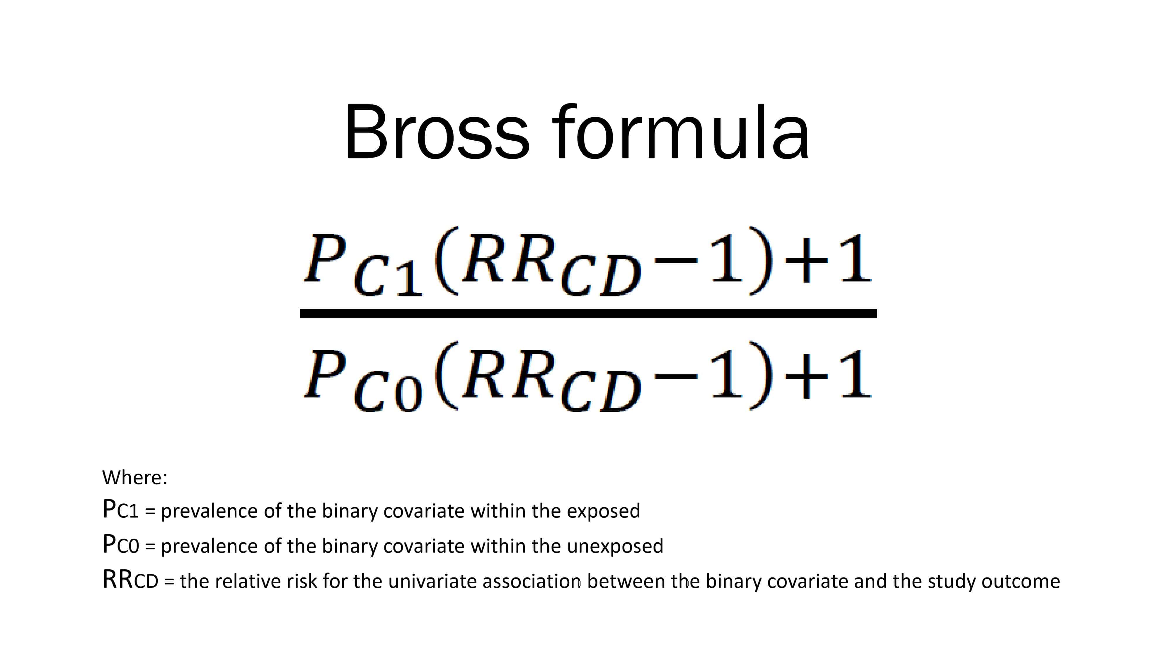
In the 4th step, we prioritize the variables based on their confounding bias, which is calculated using Bross formula. The formula considers two factors:

1. the imbalance in the prevalence of this variable across the exposure groups, and
2. the association of the variable with the outcome.

The larger the imbalance in the prevalence of a variable between exposure groups and the stronger the association of the variable with the outcome, the stronger the variable’s contribution to confounding bias. So now we have the confounding bias resulting from each of the empirical variables.

Bross formula

Exercise 2 – HDPS steps

Step 5

The 5th step is to narrow down the empirical variables to a smaller number to be included in the propensity score estimation, by selecting the variables with the highest confounding bias. There isn’t a consensus on the optimal number of variables to include, but the default is 500. In addition to these HDPS selected variables, we can add:

1. demographics (e.g., age and sex), and
2. predefined variables (any variables that we think are important confounders to include based on previous literature and expert knowledge).

By the end of this step, we have selected the variables to include in the propensity score estimation. This is the contribution of HDPS: to automatically select a large number of confounders/proxies to include in propensity score estimation. The following steps are similar to the usual propensity score estimation.

Step 6

The 6th step estimates the propensity score using logistic regression (or other selected propensity score estimation method) with the 500+ variables identified in step 5 as predictors.

Step 7

In the final step, we estimate propensity score-adjusted outcome models. So we use the propensity score estimated in step 6 to balance the exposure groups (by matching, weighing, stratification or regression adjustment) and run the outcome model.